Crypto Machine Learning: Develop a Crypto Algorithmic Trading Strategy with Python

Machine learning has become instrumental in the world of algorithmic trading strategies, utilizing numerical, categorical, and ordinal data to build simplified models of the real world. This article will leverage pycgapi, an unofficial Python wrapper for accessing the CoinGecko API, to fetch crucial market data and build an algorithmic trading strategy.

By combining Python's computational capabilities with the rich datasets provided by CoinGecko, we will apply machine learning techniques to develop, test, and implement algorithmic trading strategies in the cryptocurrency space. More specifically, we'll focus on utilizing the unsupervised machine learning algorithm called the Hierarchical Risk Parity (HRP) portfolio strategy.

Prerequisites

In this section, we've outlined the necessary background knowledge, software, and libraries you'll need, as well as steps to set up your environment, to follow along with the tutorial.

Background Knowledge

• Python Proficiency: You should be comfortable with basic programming concepts like variables, loops, and functions, as well as more advanced topics such as working with libraries and handling data.
• Understanding of Financial Markets: A basic understanding of financial markets and instruments, especially cryptocurrencies, will be beneficial.
• Mathematics and Statistics: Knowledge of basic mathematics and statistics is recommended to follow the financial analysis parts of the tutorial.

Google Colab

This tutorial utilizes Google Colab, a free cloud service that allows you to write and execute Python in your browser with zero configuration required, access to free GPUs, and easy sharing. Using Google Colab eliminates the need for local setup and ensures that everyone has access to the same computing environment, making it easier to follow along and troubleshoot.

Make sure that Google Colaboratory is added to your Google Drive account's connected apps as you see below. In your Google Drive account, click on '+New' > 'More'. If you do not see Google Colaboratory in the menu, click on '+Connect more apps'.

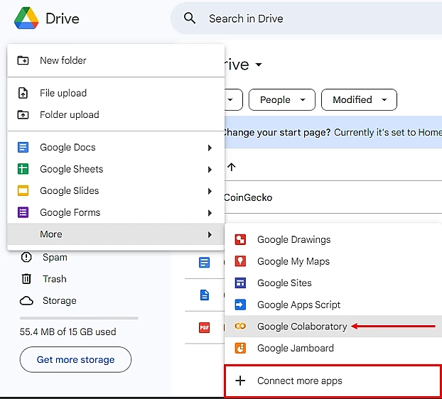
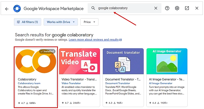
Search for "Google Colaboratory", and install it. 

Configure API Keys

For accessing crypto data and automating trades, we will be using the CoinGecko and Alpaca APIs.

• CoinGecko API: Used to fetch cryptocurrency market data.
• Alpaca API: Enables automated trading on the Alpaca platform.

Setting up your API keys for these services allows us to programmatically retrieve real-time crypto data and execute trades, which are essential components of algorithmic trading. To obtain your API keys:

• Log in to your CoinGecko account and go to the Developer's Dashboard. Click on "Add New Key". Store in a secure location.
• Log in to your Alpaca account and navigate to the Paper Trading Dashboard. Click on "Generate" in the API Keys box. After creation, your API key and secret will be displayed. It's crucial to save these securely at this point, as the secret key will not be shown again. If you lose the secret key, you'll need to generate a new pair.

Store API Keys in Google Colab Secrets

In Google Colab, click the key icon in the left side menu.

Enter the name for each key, paste the key as the value, and grant the notebook access to each key.

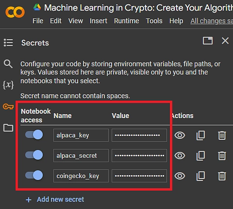
For accessing financial data, configure your API keys as follows:

Install Required Libraries

This tutorial utilizes several custom Python libraries:

• pycgapi: A client for accessing the CoinGecko API for cryptocurrency data.
• alpaca-py: The official Python library for the Alpaca trading API, enabling automated trading strategies.
• PyPortfolioOpt: Offers portfolio optimization techniques, such as mean-variance optimization.
• bt: A flexible backtesting framework for Python used to test and develop quantitative trading strategies.

Run the following commands in a Google Colab cell to install them:

Import Libraries

Once the installations are complete, import the necessary libraries using the following code. These libraries will help us manipulate data, perform financial analysis, construct portfolios, and run machine learning algorithms.

Initialize API Clients

Now, let's set up the clients needed to interact with the CoinGecko and Alpaca APIs. These clients act as the bridge between our Python code and the external services, allowing us to fetch real-time cryptocurrency data and execute trades programmatically.

For CoinGecko, we'll be using a pro API key due to the amount of data required and to operate with higher rate limits.

For Alpaca, you will need either a paper (simulated trading) or live trading API key, depending on your trading mode preference.

Initialize CoinGecko API Client

To interact with the CoinGecko API, we initialize a client that will make requests for cryptocurrency data. This data is crucial for making informed trading decisions in our algorithm.

CoinGecko API Server Status: {'gecko_says': '(V3) To the Moon!'}

Initialize Alpaca API Client

For executing trades, we use the Alpaca API client. This client will be configured for either paper trading (simulated) or live trading, based on our earlier paper setting.

Alpaca Trading Client Initialized: Paper Trading 

Investment Universe

In this section, we align the tradable cryptocurrency tickers from Alpaca with their corresponding coin IDs in CoinGecko. This alignment is crucial because Alpaca and CoinGecko use different formats for cryptocurrency tickers. For example, Alpaca uses currency pairs like "BTC/USD", whereas CoinGecko identifies cryptocurrencies by coin IDs, such as "bitcoin". By reconciling these formats, we ensure our strategy only considers cryptocurrencies that are both tradable on Alpaca and have data available on CoinGecko.

Tradable Crypto Tickers on Alpaca

First, we retrieve all tradable cryptocurrency tickers from Alpaca, focusing on those we can trade and have data for on CoinGecko.

Tradable Currency Pairs on Alpaca:

           tradable
symbol             
AAVE/USD       True
AAVE/USDC      True
AAVE/USDT      True
AVAX/USD       True
AVAX/USDC      True

Crypto Tickers from CoinGecko

Next, we match the tradable tickers from Alpaca with CoinGecko coin IDs, excluding those with a base currency of "BTC" to focus on US Dollar-based pairs.

100%|██████████| 56/56 [00:09<00:00,  5.98it/s]
Found CoinGecko IDs for 20 assets.

Collect CoinGecko Coin IDs

We collect the CoinGecko coin IDs from the search results, excluding stablecoins to focus on risky assets.

CoinGecko Coin IDs: 

aave
avalanche-2
basic-attention-token
bitcoin
bitcoin-cash
chainlink
curve-dao-token
dogecoin
ethereum
litecoin
maker
polkadot
shiba-inu
sushi
tezos
the-graph
uniswap
yearn-finance

Map CoinGecko Coin IDs to Alpaca Trading Symbols

Finally, we create a mapping between the CoinGecko coin IDs and Alpaca trading symbols for use in subsequent trading logic.

Ticker Mapping:

aave: AAVE/USD
avalanche-2: AVAX/USD
basic-attention-token: BAT/USD
bitcoin-cash: BCH/USD
bitcoin: BTC/USD
curve-dao-token: CRV/USD
dogecoin: DOGE/USD
polkadot: DOT/USD
ethereum: ETH/USD
the-graph: GRT/USD
chainlink: LINK/USD
litecoin: LTC/USD
maker: MKR/USD
shiba-inu: SHIB/USD
sushi: SUSHI/USD
uniswap: UNI/USD
usd-coin: USDC/USD
tether: USDT/USD
tezos: XTZ/USD
yearn-finance: YFI/USD

Fetching Real-time & Historical Crypto Price Data

Use the CoinGecko API to fetch real-time and historical crypto price data. This is essential for the analysis underlying our trading strategy.

Earliest Start Dates

The availability of historical data is assessed to ensure each cryptocurrency in our selection has sufficient historical data for analysis. Use this information to assess whether you should to omit any assets whose earliest start date is too recent.

100%|██████████| 18/18 [00:13<00:00,  1.37it/s]

Earliest Data Start Dates:

 the-graph                2020-12-17
aave                     2020-10-03
avalanche-2              2020-09-22
uniswap                  2020-09-17
sushi                    2020-08-28
polkadot                 2020-08-19
curve-dao-token          2020-08-14
shiba-inu                2020-08-01
yearn-finance            2020-07-18
tezos                    2018-07-03
maker                    2017-12-20
chainlink                2017-11-09
bitcoin-cash             2017-08-02
basic-attention-token    2017-06-08
ethereum                 2015-08-07
dogecoin                 2013-12-15
bitcoin                  2013-04-28
litecoin                 2013-04-28
Name: Start Dates, dtype: object

Current Prices

We download current market prices for each selected cryptocurrency, providing a current view of market conditions.

Current Prices:

                     usd
AAVE/USD     102.730000
AVAX/USD      38.930000
BAT/USD        0.270338
BTC/USD    53392.000000
BCH/USD      270.950000
LINK/USD      18.960000
CRV/USD        0.599837
DOGE/USD       0.086983
ETH/USD     3152.620000
LTC/USD       71.140000
MKR/USD     2092.800000
DOT/USD        7.990000
SHIB/USD       0.000010
SUSHI/USD      1.570000
USDT/USD       1.000000
XTZ/USD        1.130000
GRT/USD        0.293909
UNI/USD       10.690000
USDC/USD       1.000000
YFI/USD     8325.900000

Historical Data

We download historical price, market capitalization, and trading volume data for each selected cryptocurrency. This dataset is crucial for analyzing market behavior over the specified period.

100%|██████████| 20/20 [00:12<00:00,  1.63it/s]

Historical Prices:

                                bitcoin  bitcoin-cash  chainlink  \
timestamp                                                          
2022-11-21 00:00:00+00:00  16304.076856    104.914267   5.780015   
2022-11-22 00:00:00+00:00  15814.335281    103.401328   5.878893   
2022-11-23 00:00:00+00:00  16171.628978    108.902578   6.386520   
2022-11-24 00:00:00+00:00  16608.009985    114.523828   6.721798   
2022-11-25 00:00:00+00:00  16596.035758    116.688272   6.833340   

                           curve-dao-token  dogecoin  
timestamp                                             
2022-11-21 00:00:00+00:00         0.512044  0.077732  
2022-11-22 00:00:00+00:00         0.501516  0.075124  
2022-11-23 00:00:00+00:00         0.633928  0.078690  
2022-11-24 00:00:00+00:00         0.688066  0.082338  
2022-11-25 00:00:00+00:00         0.689696  0.081835  

Categorical Data

Finally, categorical information for each cryptocurrency is collected. This data helps to understand the diversification and exposure of the portfolio across different cryptocurrency categories.

100%|██████████| 20/20 [00:09<00:00,  2.08it/s]

Data Processing

This section outlines the steps to normalize, analyze, and visualize the historical cryptocurrency data, setting a foundation for machine learning analysis.

Normalize Prices for Comparative Analysis

Given the significant price differences across cryptocurrencies, we normalize all prices to start at $1. This approach enables a direct comparison by equalizing the initial investment across all assets.

Compute Historical Returns

We calculate daily and cumulative returns from the normalized prices, which serve as key metrics for evaluating asset performance.

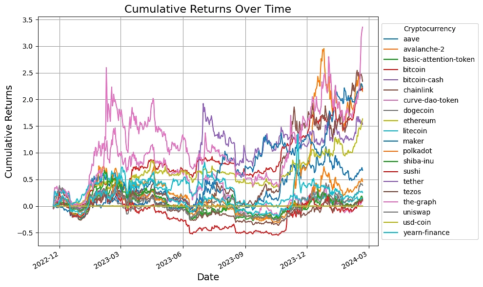
Visualize Cumulative Returns

Visualizing the cumulative returns of selected cryptocurrencies not only brings the data to life but also aids in the identification of standout performers and underperformers within our investment universe.

Prepare Data for Machine Learning

Prior to machine learning analysis, we standardize the historical returns. This normalization ensures that all data features contribute equally to the analysis, improving algorithm performance.

Standardized Historical Returns:

                            bitcoin  bitcoin-cash  chainlink  curve-dao-token  \
timestamp                                                                       
2022-11-22 00:00:00+00:00 -1.451238     -0.430926   0.357041        -0.492130   
2022-11-23 00:00:00+00:00  0.874272      1.263095   2.156707         3.000000   
2022-11-24 00:00:00+00:00  1.068304      1.223372   1.276908         1.909221   
2022-11-25 00:00:00+00:00 -0.155862      0.403770   0.343712         0.027544   
2022-11-26 00:00:00+00:00 -0.314597     -0.667662   0.001589        -0.341132   

                           dogecoin  
timestamp                            
2022-11-22 00:00:00+00:00 -1.023868  
2022-11-23 00:00:00+00:00  1.392055  
2022-11-24 00:00:00+00:00  1.359091  
2022-11-25 00:00:00+00:00 -0.205570  
2022-11-26 00:00:00+00:00  2.897963  

Algorithmic Trading Strategy: What is Hierarchical Risk Parity (HRP)?

The Hierarchical Risk Parity (HRP) method, introduced in López de Prado (2016), uses hierachical clustering to group assets, not by past returns, but by the similarity in their price series. HRP aims to minimize estimation errors found in conventional portfolio optimization methods by constructing a diversified portfolio that considers the hierarchical relationships between assets. HRP's effectiveness lies in its robustness to market shifts, often outperforming classical diversification techniques.

Hierarchical Risk Parity

We start by structuring our assets using hierarchical clustering. This method begins with each asset as a separate cluster and merges them iteratively based on their correlations. The outcome reveals natural groupings in the data, aiding in diversified portfolio construction.

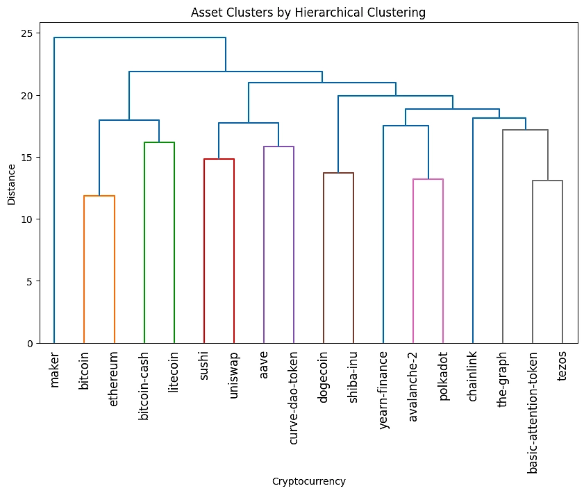
The dendrogram shows how assets link together, with closer branches indicating similar price behaviors. For instance, Bitcoin and Ethereum cluster early, indicating correlated price movements. Conversely, Maker's distinct branch suggests its price behavior is less correlated with the others.

Portfolio Optimization

In the portfolio optimization phase, Hierarchical Risk Parity (HRP) is employed to integrate the clustering results into the asset allocation process. This method accounts for the inherent structure and relationships between assets identified through hierarchical clustering. A crucial step in this process involves computing a risk model using a covariance matrix. The Covariance Shrinkage method, specifically the Ledoit-Wolf shrinkage, is applied to historical returns, which tempers estimation errors by combining the sample covariance with a structured estimator, or "shrinkage target," resulting in a more stable and robust covariance matrix. The HRP model uses this refined covariance matrix to determine the optimal asset weights, aiming for a diversified portfolio that is less sensitive to estimation errors and more attuned to underlying market structures.

HRP Optimized Portfolio:

                      Optimized Weights
Asset                                  
bitcoin                           8.68%
polkadot                          7.26%
litecoin                          7.14%
ethereum                          7.02%
dogecoin                          6.85%
tezos                             6.74%
shiba-inu                         6.58%
uniswap                           6.26%
basic-attention-token             6.24%
aave                              5.56%
chainlink                         5.11%
yearn-finance                      4.6%
maker                             4.22%
avalanche-2                       4.17%
curve-dao-token                   3.89%
bitcoin-cash                      3.76%
sushi                             3.16%
the-graph                         2.77%


Expected annual return: 45.7%
Annual volatility: 43.4%
Sharpe Ratio: 1.01

The output of this optimization presents the asset weights guided by the HRP approach and the robust covariance estimation. The performance metrics, which include expected annual return, annual volatility, and Sharpe Ratio, provide a comprehensive view of the portfolio's risk-reward profile.

Categorical Weighting

Finally, we use categorical data to evaluate our portfolio's exposure across various cryptocurrency categories.

Categorical Weights:

Decentralized Finance (DeFi)    35.56%
Smart Contract Platform         34.06%
Layer 1 (L1)                    30.37%
Proof of Stake (PoS)            27.96%
Governance                      27.68%
Proof of Work (PoW)             26.43%
Meme                            13.43%
Layer 0 (L0)                     7.26%
Name: Category Weights, dtype: object

Note: Categories can overlap so weights unlikely to total 100%.

The portfolio's largest categorical weighting is in Decentralized Finance (DeFi) at 35.56%, closely followed by Smart Contract Platforms at 34.06%. Both Layer 1 protocols and Proof of Stake mechanisms also hold significant weights, emphasizing the portfolio's tilt towards foundational blockchain technologies and governance systems.

Backtesting Strategy

Backtesting is a crucial step in evaluating the performance of any trading strategy. It allows us to simulate how the strategy would have performed in the past, providing insights into potential future performance. This section outlines the backtest of a Hierarchical Risk Parity (HRP) strategy against other benchmark strategies, including Equal Weighted (EW), Equal Risk Contribution (ERC), and Monte Carlo simulation of randomly generated portfolios.

Strategy Logic

Hierarchical Risk Parity (HRP) Strategy

The HRP strategy aims to optimize asset allocation by considering the hierarchical structure of asset correlations, thus potentially reducing portfolio volatility and improving returns. The WeighHRP class, defined below, implements this strategy by selecting assets and rebalancing the portfolio based on a lookback period.

Equal Risk Contribution (ERC) Strategy

The ERC strategy seeks to allocate portfolio weights in a way that each asset contributes equally to the portfolio's risk, aiming for a more balanced risk distribution across assets.

Backtest Engine

The backtest engine simulates the performance of these strategies over a specified period. It uses historical price data to execute trades according to each strategy's logic and calculates the portfolio's value over time.

Run the Backtest

To initiate the backtest, we set the number of simulations for random portfolios and the lookback period for rebalancing.

The risk-free rate is also defined to calculate the excess return used for risk-adjusted performance.

[*********************100%%**********************]  1 of 1 completed
Average Risk-Free Rate: 3.95%

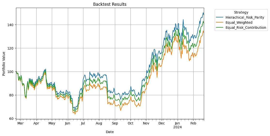
Run all backtests and plot the performance results of a $100 starting value portfolio for each backtest.

100%|██████████| 3/3 [00:01<00:00,  2.23it/s]
100%|██████████| 1/1 [00:00<00:00, 7345.54it/s]
100%|██████████| 1/1 [00:00<00:00, 10866.07it/s]
100%|██████████| 1/1 [00:00<00:00, 11214.72it/s]
100%|██████████| 1000/1000 [02:17<00:00,  7.29it/s]

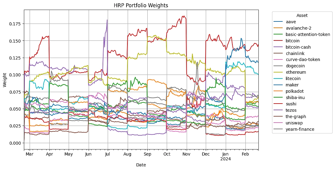
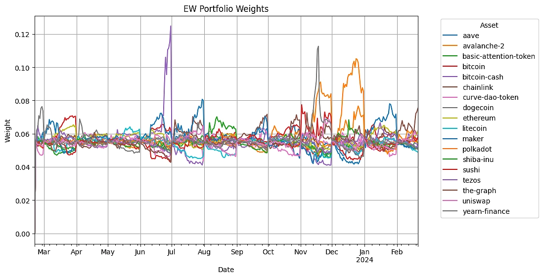
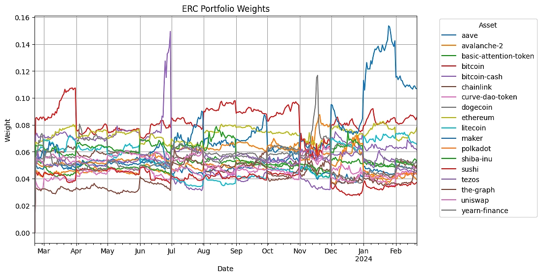
Plot Security Weights

Visualizing the weight allocations over time provides insights into how each strategy changes to market conditions. It helps in understanding the diversification and risk management approach of each strategy.

Backtest Results

After running the backtests, we compile and display the performance statistics for each strategy. This includes measures such as total return, annualized return, maximum drawdown, Sharpe ratio, and others. Comparing these metrics across strategies helps in evaluating their relative performance and risk characteristics.

Backtested Portfolios:

• HRP: Hierarchical Risk Parity
• EW: Equal Weighted
• ERC: Equal Risk Contribution
• ARP: Aggregate Random Portfolio

During the one-year sample period from February 20, 2023, to February 21, 2024, the Hierarchical Risk Parity (HRP) strategy outperformed the Equal Weighted (EW), Equal Risk Contribution (ERC), and Aggregate Random Portfolio (ARP) strategies in terms of total return, with HRP achieving a 48.35% return. It also exhibited a Compound Annual Growth Rate (CAGR) of 48.23% and a maximum drawdown of -33.78%. While the HRP strategy showed a notable Calmar Ratio of 1.43 and the highest Monthly Sharpe Ratio of 1.25 among the strategies, indicating a favorable risk-adjusted return during the sample period, it is important to recognize that these results are specific to the timeframe analyzed. The performance of the HRP strategy, compared to the others, underscores its effectiveness in this particular context without necessarily implying overall superiority across all market conditions or time periods.

Monte Carlo Hypothesis Test

In the hypothesis test, we are examining whether the Hierarchical Risk Parity (HRP) strategy's performance, as measured by the monthly Sortino ratio, is significantly better than what could be expected by random chance from a selection of portfolios. The null hypothesis (H₀) and alternative hypothesis (H_a) are defined as follows:

H0: Strategy's return ≤ 1,000 random portfolios. (μstrategy ≤ μrandom)
Ha: Strategy's return > 1,000 random portfolios. (μstrategy > μrandom)

Here, μ_strategy is the mean monthly Sortino ratio of the investment strategy, and μ_random is the mean monthly Sortino ratio of the random portfolios.

Result: The portfolio outperformed the sample of randomly generated portfolios.

T-statistic: 18.0693
P-value (one-tailed): 0.0000
Significance Level: 0.05

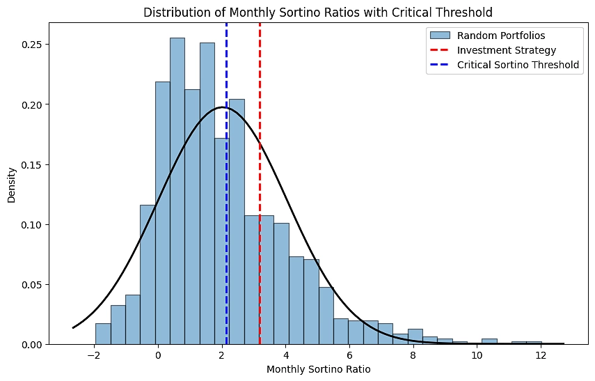
Upon running the test, the results display a p-value of 0.0000 and a t-statistic of 18.0693. If we reject the null hypothesis, we are asserting that there is sufficient evidence to claim that the investment strategy has outperformed the random portfolios with a confidence level of 95%. The plot further substantiates this finding, showing the investment strategy's Sortino ratio significantly to the right of the critical Sortino ratio threshold and the distribution of the random portfolios.

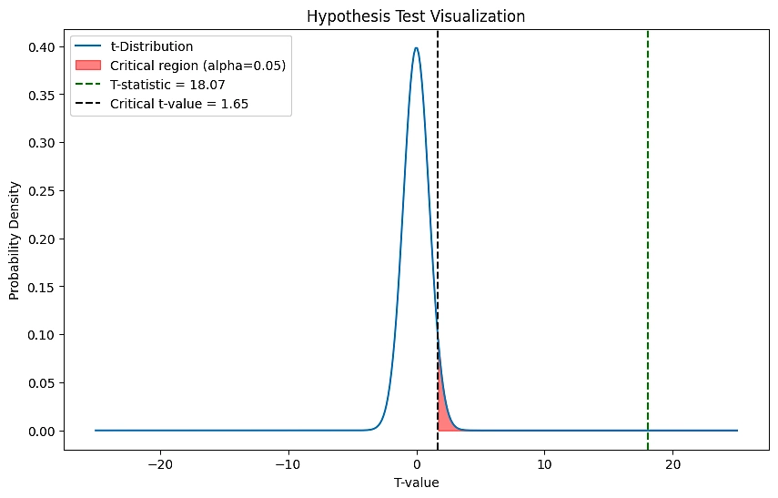
The plot visualizes the results of the hypothesis test for the Hierarchical Risk Parity (HRP) strategy's performance. The blue curve represents the t-distribution of t-values obtained from the Monte Carlo simulation. The red shaded area to the right of the black dashed line signifies the critical region for our alpha level of 0.05, where any t-statistic falling within this region would lead us to reject the null hypothesis. Our observed t-statistic, indicated by the green dashed line, falls well within the critical region, affirming that the HRP strategy's performance is statistically significantly greater than that of the random portfolios. The critical t-value of 1.65 is the threshold above which we reject the null hypothesis, and our t-statistic of 18.07 vastly exceeds this, providing strong evidence against the null hypothesis in favor of the alternative.

Automating Strategy

This section introduces a trading bot that automatically executes the Hierarchical Risk Parity strategy, converting targeted allocations into market orders while managing existing positions and respecting minimum trade thresholds. The bot also features a preview mode to validate trades before execution.

Trading Bot

The function create_positions_dataframe converts the account positions into a Pandas DataFrame. This standardized format is essential for the trading bot to assess current holdings against target allocations.

The preview_mode flag allows users to test the trading bot without executing real trades, providing a safeguard and a means to validate the bot's logic before live operation. If preview_mode is set to False, then the trading bot will execute live orders. Use with caution.

The min_trade_value is set to $100, indicating that the bot will ignore any trades below this amount to ensure that transactions are economically viable.

Here we initialize our trading bot, fetching current account details and holdings. It assesses the portfolio's value, cash availability, and buying power. Based on the optimized weights from our strategy, the bot prepares a list of trades, considering the minimum trade value threshold to avoid executing economically insignificant trades. The trading bot then simulates the execution of these trades, providing an overview of buy and sell orders. This simulation allows for a final review before live trading, ensuring alignment with our strategy and capital allocation rules.

Starting Trading Bot...

Portfolio Value: $102,198.99
Cash: $14,678.53
Buying Power: $29,357.06

Account Holdings: 
                    qty               side  market_value    cost_basis
symbol                                                                
AAVE/USD      53.031986  PositionSide.LONG   5449.036580   4873.639530
AVAX/USD      56.150439  PositionSide.LONG   2166.845424   2175.267990
BAT/USD    13704.653261  PositionSide.LONG   3705.436739   3453.435575
BCH/USD       20.679385  PositionSide.LONG   5605.560950   5374.841049
BTC/USD        0.304311  PositionSide.LONG  16271.957289  15619.655041
CRV/USD    10941.174129  PositionSide.LONG   6583.960944      0.000000
DOGE/USD   34293.311273  PositionSide.LONG   2987.156601   2956.426365
DOT/USD      463.152266  PositionSide.LONG   3719.112695      0.000000
ETH/USD        2.761884  PositionSide.LONG   8713.744512   8071.661684
GRT/USD     7204.676907  PositionSide.LONG   2120.480507   1720.671372
LINK/USD     277.058115  PositionSide.LONG   5253.215799   5090.194804
LTC/USD      101.623754  PositionSide.LONG   7216.099548   7009.420266
SUSHI/USD   2899.258768  PositionSide.LONG   4541.109008   3664.692075
UNI/USD      682.816928  PositionSide.LONG   7777.284814   5011.261719
XTZ/USD     4775.295230  PositionSide.LONG   5409.454436      0.000000

Preparing Trades...

100%|██████████| 18/18 [00:00<00:00, 4038.16it/s]

Previewing Trades...

Preview sell order for BTC/USD: Notional $7,400.06
Preview sell order for ETH/USD: Notional $1,535.29
Preview sell order for UNI/USD: Notional $1,379.63
Preview sell order for CRV/USD: Notional $2,612.51
Preview sell order for BCH/USD: Notional $1,760.83
Preview sell order for SUSHI/USD: Notional $1,314.69
Preview buy order for DOT/USD: Notional $3,700.53
Preview buy order for DOGE/USD: Notional $4,011.43
Preview buy order for XTZ/USD: Notional $1,474.67
Preview buy order for SHIB/USD: Notional $6,725.72
Preview buy order for BAT/USD: Notional $2,669.74
Preview buy order for AAVE/USD: Notional $231.18
Preview buy order for YFI/USD: Notional $4,696.04
Preview buy order for MKR/USD: Notional $4,313.82
Preview buy order for AVAX/USD: Notional $2,091.79
Preview buy order for GRT/USD: Notional $711.45

Total Trades: 16
Sell Trades: 6
Buy Trades: 10

Done!

CoinGecko's Content Editorial Guidelines

CoinGecko’s content aims to demystify the crypto industry. While certain posts you see may be sponsored, we strive to uphold the highest standards of editorial quality and integrity, and do not publish any content that has not been vetted by our editors.

Learn more

Nathan Ramos, CFA

Nathan Ramos is a financial software developer with a focus on Python-based financial analysis, quantitative strategies, and automated trading algorithms, holding the Chartered Financial Analyst designation. His work bridges traditional finance with emerging financial technologies, enhancing tools for cryptocurrency data accessibility and trading efficiency. He is also the creator of pycgapi, an unofficial Python wrapper for CoinGecko API that simplifies access to cryptocurrency data. Follow the author on Twitter @nathanramoscfa